Study Site
The study site is located in Ft. Benning in the centre of Georgia on the geographical Fall Line, United States (Fig. 1). The installation covers two major ecological provinces: the Sandgills in the northeastern two-thirds of the installation, and the Upper Loam Hills in the southwestern one-third. The terrain is rolling and ranges in elevation from 58 to 225 m above sea level (USAIC 2006). The climate is classified as warm humid temperate with hot, humid summers and mild winters. Mean annual precipitation is 1240 mm and is evenly distributed throughout the year (National Data Center, Asheville, NC). Major soil textures are loamy sand, sandy loam, and sandy clay loam.
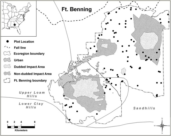
Figure 1. The location of the study site.
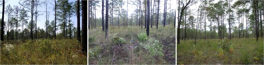
Figure 2. Study sites representing each type of stands.
Field Survey
We measured the diamter at breast height (DBH; 1.3 m height) and recorded the species of each tree > 5 cm DBH in each plot. For loblolly pines, we evaluated crown condition including crown vigor class (CVC). CVC was determined mainly by live crown ratio, crown dieback (%; crown), and crown density (%; relative to the surrounding healthy trees) following the USDA Forest Service Health Monitoring protocol (USDA Forest Service 1999). CVC assigns each tree a "grade" to describe canopy health (1 = goodn, 2 = fair, 3 = poor) and was used as an indicator of tree health (CVC 1= crown ratio > 35 percent, crown dieback < 5 percent, and crown density > 80 percent; CVC3 = crown density < 35 percent, crown dieback > 50 percent, and crown density < 20 percent; and all other trees were classified as CVC2)(Table 1). We also measured crown light exposure (range 0 to 5; 0 is the lowest light exposure and 5 is full exposure) and crown position (1 = super-dominant, 2 = dominant and codominant, and 3 = intermediate and overtopped), crown density and crown dieback. Additionally, any visible symptoms of poor health or damage (e.g., fusiform rust, physical scar, stem canker, and excessive cone production ) were also noted. The center of each plot was mapped using global positioning system, and slope and aspect of each plot were recorded.
Tree ring samples were cored from 5 live and 5 dead trees in each plot. When every dead tree in a plot were fallen or not appropriated for coring, it was necessary to find another tree near the plot. We took two cores (south and north side) of each tree at breat height using an increment borer.
Tree ring samples were cored from 5 live and 5 dead trees in each plot. When every dead tree in a plot were fallen or not appropriated for coring, it was necessary to find another tree near the plot. We took two cores (south and north side) of each tree at breat height using an increment borer.
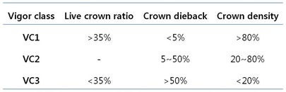
Table 1. How to calculate vigor classes.
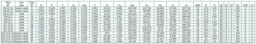
Table 2. Master data table.

Table 3. Tree ring widths data.

Table 4. My denpendent and independet variables.
Data Analysis
To find out the difference between independent variables in vigor class 1 and vigor class2, I divided each independent variable into two groups: vigor class 1 and vigor class 2. Then I drew barplots and boxplots to visualize them to test assumptions of Student T-tests in R. I also did multiple linear regression analysis to find which independent variables are related to my dependent variable, vigor class.
Each tree core was measured with Velmex measuring system with a resolution of 0.001 mm. Prior to further analysis using tree ring series, we plotted growth curves to cross-date each tree ring and the curves were used to evaluate missing rings or false rings in the cores (Douglas, 1941). After measuring the ring widths, we ran COFECHA to check the quality of dating (Holmes, 1983). Then the master chronology representing all the trees in the study sites was built after the tree ring measurements were standardized to remove the autocorrelation component in the time series (Cook and Holmes 1986, Speer 2010).
Each tree core was measured with Velmex measuring system with a resolution of 0.001 mm. Prior to further analysis using tree ring series, we plotted growth curves to cross-date each tree ring and the curves were used to evaluate missing rings or false rings in the cores (Douglas, 1941). After measuring the ring widths, we ran COFECHA to check the quality of dating (Holmes, 1983). Then the master chronology representing all the trees in the study sites was built after the tree ring measurements were standardized to remove the autocorrelation component in the time series (Cook and Holmes 1986, Speer 2010).
